How scientists map a seafloor they cannot see

In the 1950s, Marie Tharp worked at a drawing table while research ships crossed the Atlantic. The ships returned with long strips of depth measurements, not photographs. Tharp plotted those depth readings, called soundings, as cross-sections of the seafloor and found a valley running through the crest of a vast underwater mountain chain. A landscape hidden beneath kilometres of water had begun to reveal a geological argument: the ocean floor was not a featureless basin.

Her maps made the Mid-Atlantic Ridge and its central valley visible. This strengthened the emerging case for seafloor spreading, where new crust forms and moves outward. It also supported plate tectonics, the movement of large pieces of Earth’s outer shell. Yet Tharp was also explicit about the gaps. In areas without soundings, she extended the patterns seen in measured areas to estimate what might lie between them and revised the picture when new tracks arrived. Her first-person account at Columbia's Lamont-Doherty Earth Observatory describes the work as connecting profiles across an incomplete canvas.

Modern maps contain vastly more data, but they still depend on the same discipline: distinguish what an instrument measured from what a model inferred.

First, turn an echo into distance

Light and radar are rapidly absorbed in seawater, while sound can travel much farther. Active sonar sends a sound pulse downward and listens for its echo. If the round trip takes four seconds and sound is assumed to travel at 1,500 metres per second, the travelled path is 6,000 metres. Divide by two to account for the outward and return journeys, and the estimated depth is 3,000 metres.

The compact equation is depth = sound speed × round-trip time ÷ 2. The arithmetic is simple; obtaining reliable inputs is not. NOAA's seafloor-mapping explainer traces the progression from weighted lead lines, through single-beam echo sounders, to multibeam systems.

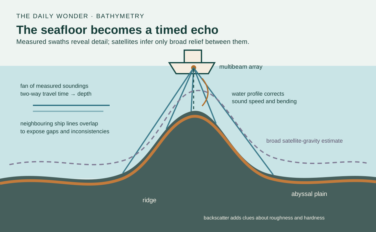
A single beam is like taking one depth beneath the ship. A multibeam echosounder sends many narrow beams in a fan across the vessel's track, measuring a strip called a swath. As the ship follows neighbouring lines, overlapping swaths build a set of measured seafloor points, called a point cloud. Mapping specialists arrange those points into a grid of depths. This bathymetric grid is the underwater equivalent of a land-height map. NOAA explains the fan geometry and processing.

Deeper water creates a trade-off. A fixed beam angle covers a wider strip as the bottom becomes farther away, so a ship can survey more width per pass. But the individual footprints spread out too, and fine detail is harder to resolve. For close inspection, sonar can be carried nearer the bottom on an autonomous vehicle, remotely operated vehicle or towfish.

The ocean bends the ruler

The familiar value of 1,500 metres per second is an approximation, not a universal constant. Sound speed changes with temperature, salinity and pressure. Those properties vary with depth, so a beam sent at an angle through the layers can change direction. This bending is called refraction. A wrong speed profile therefore shifts both the calculated depth and the horizontal position of an outer beam.

Mapping teams measure the water column. An expendable bathythermograph, or XBT, falls from a ship while sending temperature measurements through thin wires. Combined with salinity information, the observations produce a sound-speed profile that software applies to the sonar data. NOAA's XBT guide explains why this correction matters.

The ship is moving too. It rises and falls, rolls, pitches and changes heading. The sonar head has a position and orientation relative to the navigation sensors. Tides change the reference water level. Processing must account for these effects, reject weak or spurious returns, compare overlapping lines and calibrate timing and alignment. A colourful surface is therefore not a direct picture; it is the end of a measurement chain.

Shape and texture are different measurements

Travel time mainly supplies bathymetry, the geometry of depth. The strength of the returned echo supplies backscatter. Hard rock generally sends back a stronger signal than soft mud; roughness and beam angle also influence the return. Backscatter can therefore suggest changes in bottom character, but it is not a photograph and does not identify a material with certainty.

Scientists compare acoustic patterns with video, sediment samples and other observations. NOAA's backscatter guide explains how depth and echo strength complement each other. This distinction matters: two places can have similar depth but very different habitats, while one material can produce different returns under different geometries.

Satellites sketch the large shapes

A satellite radar altimeter cannot send its signal through kilometres of seawater to the bottom. Instead, it measures the sea surface. A massive underwater mountain slightly changes local gravity, which subtly alters the height and shape of the water above it. Combining these surface measurements with ship soundings lets scientists estimate the seafloor’s broad mountains, valleys and plains.

That global view is powerful but indirect. NOAA describes satellite-derived bathymetry as lower resolution than modern ship sonar: it can reveal large structures and guide surveys, not replace close measurement. Compare the two scales in NOAA's mapping overview. A smooth-looking global map may therefore combine dense measured swaths, sparse tracks and gravity-based estimates.

As of April 2026, NOAA reported that 28.7 percent of the global seafloor had been mapped with modern high-resolution technology. That does not mean the remaining ocean is a blank colour. It means it lacks mapping that meets the modern multibeam standard. NOAA separates high-resolution mapping from direct visual exploration, which covers a far smaller area.

A map is also a record of confidence

Seafloor maps guide ships, tsunami and coastal-hazard modelling, habitat studies, cable routes, geological research and the choice of places to send deep-sea vehicles. Their value depends on knowing the origin, resolution and age of the data, not merely admiring a shaded relief image.

Tharp's hand-drawn profiles and today's multibeam grids belong to the same intellectual tradition. Each converts indirect measurements into a landscape while keeping track of uncertainty. The ocean floor becomes visible not because water has turned transparent, but because scientists learn what an echo can say, what gravity can suggest, and where the map must still admit: we have not measured this closely yet.