How ocean currents move heat

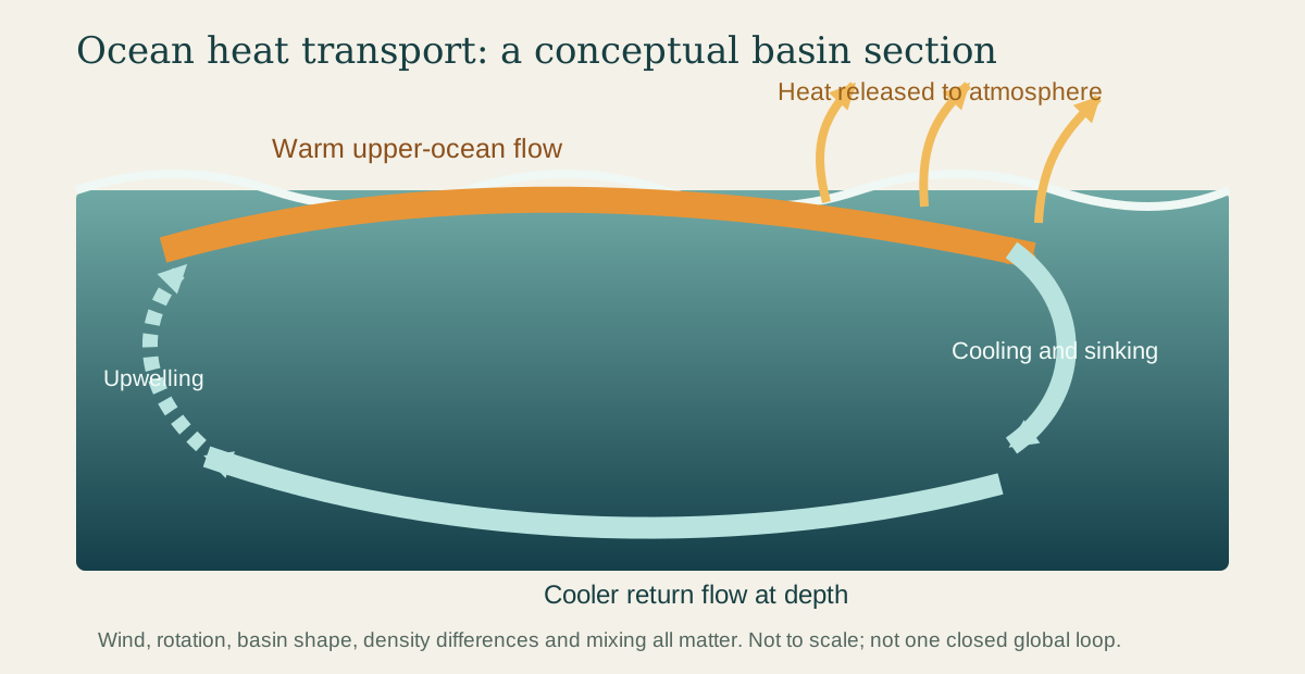
On a winter map of the North Atlantic, water leaving the tropics may still carry the memory of intense sunlight. The heat is invisible, but the moving water can release some of it to the air thousands of kilometres from where it entered the ocean.

This helps Earth soften the contrast between a hot equator and cold poles. The atmosphere performs much of the same planetary work, and neither system follows a simple route. Ocean currents weave through basins, turn at continents, plunge beneath other water, rise again and spin into eddies, swirling patches of water. They form a moving, three-dimensional network.

Why there is heat to move

Sunlight does not warm Earth evenly. On average, low latitudes receive more solar energy than high latitudes. The tropics would keep accumulating energy and the poles would keep losing it if the atmosphere and ocean did not transport heat between regions.

Water is unusually good at storing thermal energy. A current therefore moves more than seawater, salt and living organisms: it carries heat content. When warm water travels poleward, cools and gives energy to the atmosphere, it contributes to a transfer that can influence winds, rainfall and regional temperatures. NOAA describes currents as part of the mechanism that carries warm water away from the equator and cold water away from the poles. NOAA's current overview identifies wind, tides and water-density differences as the main drivers.

The word “warm” is relative. A current does not need to feel tropical to transport heat. What matters is the quantity of water moving and its temperature compared with water returning in the other direction.

Wind draws the surface map

Persistent winds drag on the upper ocean. Because Earth rotates, moving water follows a curved path relative to Earth’s surface. This is the Coriolis effect. Continents also redirect the flow. Together these influences organize great rotating systems called gyres.

The flow is uneven. On the western side of many ocean basins, currents such as the Gulf Stream and Kuroshio become relatively narrow, deep and swift. On the eastern side, the return flow is generally broader and slower. Eddies peel away, fronts wander and seasonal winds reshape parts of the pattern. The NASA visualization linked below makes that restless texture visible rather than drawing currents as fixed blue arrows.

Surface circulation also moves water vertically. Winds can push surface water away from a coast or region, allowing colder, nutrient-rich water to rise in upwelling. Elsewhere, water converges and sinks. These vertical exchanges help connect the sunlit surface to the enormous volume below.

Temperature and salt change density

Density is mass per unit volume: denser water has more mass packed into the same space. Seawater density depends partly on temperature and salinity, how much dissolved salt it contains. Cooling generally makes seawater denser; adding salt does too. In some high-latitude regions, surface water cools, becomes dense enough to sink, and helps form deep water masses.

Those masses spread through the ocean interior. Eventually, mixing and wind-driven upwelling bring deep water back toward the surface. NOAA calls the combined deep and surface circulation the global ocean conveyor belt. Its overview follows cooling, sinking, deep flow and eventual return, while the NOAA currents tutorial separates wind-driven surface flow from density-related circulation.

The conveyor is a useful first picture, but not one continuous belt driven from a single point. Winds help drive overturning; water takes branching paths; mixing matters; and different depths move on different timescales. Oceanographers plot north–south flow at different depths in latitude–depth sections. They call the combined upper and lower flows overturning circulation. This does not mean that every pocket of water follows one neat route around the globe.

A chart born from travel time

Long before satellites could measure sea-surface height, sailors knew that the Atlantic contained a powerful current. In the eighteenth century, Benjamin Franklin investigated why British mail packets took longer to sail westward than experienced American vessels. He consulted Timothy Folger, a Nantucket mariner and whaler who knew the current's route.

Folger sketched the flow and Franklin helped publish the chart. The Library of Congress record identifies the map as authorized by Franklin and Folger; another Library of Congress description credits Folger's original sketch. Franklin asked the question; Folger supplied practical knowledge gained at sea.

Their chart could help ships avoid fighting the current. It also expressed a larger idea: the ocean had persistent structures that could be mapped, measured and used.

How we see an invisible transport

Modern observing systems view different pieces of the circulation. Satellites measure sea-surface temperature and tiny variations in sea-surface height; the slope of the ocean surface helps reveal pressure differences related to current flow. Drifting instruments follow water near the surface. Profiling floats repeatedly descend and rise, measuring temperature and salinity through the upper ocean. Instruments anchored in place, called moorings, and surveys from ships provide records across important parts of the flow.

Scientists combine these observations with physical models. NASA's Perpetual Ocean visualization, for example, uses a model constrained by satellite and in-water observations and shows surface flow from June 2005 to December 2007. NASA notes that the underlying ECCO2 system represents all depths, although only the surface appears in that artwork. The visualization and its data description are available from NASA's Scientific Visualization Studio.

What a current does and does not do

It is tempting to credit one famous current with an entire regional climate. The Gulf Stream certainly carries heat northeastward, but western Europe's climate cannot be reduced to a single oceanic cause. Atmospheric circulation also moves enormous quantities of heat, and prevailing winds, geography and the ocean interact.

Nor does a change in one current imply that all ocean circulation has “stopped.” Surface gyres and deep overturning have different drivers and can change in different ways. Measurements must specify which flow, depth, region and time period they describe.

Sunlight adds heat to the ocean, currents carry it elsewhere, and the sea exchanges energy with the atmosphere. Water beside a cold coast may therefore carry heat from a distant region. A current connects places through moving water and the energy it carries.